NOTE 15B: Imagine that a large population is reduced to a much smaller size, so that most variation is lost. Then, the distribution of allele frequencies among the loci that remain polymorphic (a fraction 6p0q0e–t/2Ne) is approximately uniform. This is a quite different prediction from the case when mutation and drift have reached an equilibrium (as in the standard neutral theory) and so can be used to distinguish these alternatives. We will see examples where the distribution of allele frequencies is used in this way in Chapter 19.
NOTE 15C: This relationship was derived by Clayton and Robertson (1955); Lynch and Hill (1986) developed the neutral theory of quantitative variation further.
NOTE 15D: It is interesting that even if random drift eliminates all variation, the trait mean is unlikely to change by more than 2 s.d., or 2 ![]() (i.e., by more than 2
(i.e., by more than 2![]() times the s.d. of the distribution of initial breeding values).
times the s.d. of the distribution of initial breeding values).
NOTE 15E: This is the harmonic mean population size.
NOTE 15F: Under the Wright–Fisher model, the distribution of the number of offspring is close to Poisson. A Poisson distribution is often assumed for convenience, but, usually, the actual variance in offspring number is greater than in a Poisson.
NOTE 15G: The fact that when queens mate only once, daughters are more closely related to each other than daughters are to their mothers is thought to favor the evolution of sociality in haplodiploids (see Box 21.2). Note that the relatedness coefficient, r, which plays a key role in Hamilton’s theory of kin selection, is twice the coefficient of kinship calculated here (p. 601).
NOTE 15H: We assume here a very large population and count only identity due to recent ancestry; if we go back far enough, then all genes are IBD. We have also assumed that inbreeding does not “run in families.”
NOTE 15I: This sum actually simplifies neatly, because
![]()
So, we have
NOTE 15J: This justifies the statement in the text (p. 423) that with a large sample, it takes on average the same time to coalesce from many lineages down to two as from two lineages down to one.
NOTE 15K: More generally, the sum 1 + 1/2 + ... + 1/(N – 1) is close to loge(N) + 0.577, and so the expected number of segregating sites increases logarithmically with the size of the sample.
NOTE 15L: Tajima’s D statistic is based on a comparison between the pairwise diversity and the number of segregating sites and is widely used for detecting deviations from the standard neutral model (see Chapter 19, Web Notes).
NOTE 15M: How accurately does the infinite sites model describe this sample? The basic assumption of the infinite sites model is that every mutation is at a new site. One consequence of this is that each SNP segregates for only two alleles: If three or four segregate, then there must have been multiple mutations at that site. In this case, there are expected to be 283 segregating sites out of 10,000 bp. Therefore, the chance that any one mutation occurs at a site that is already segregating is 283/10,000 = 0.0283. However, the chance that all 283 are at different sites is
So, although the approximation is very accurate for any particular site, there are likely to be a few sites with multiple mutations. This calculation is similar to finding the chance that 20 people all have different birthdays; there is about 40% chance that some will in fact share the same birthday.
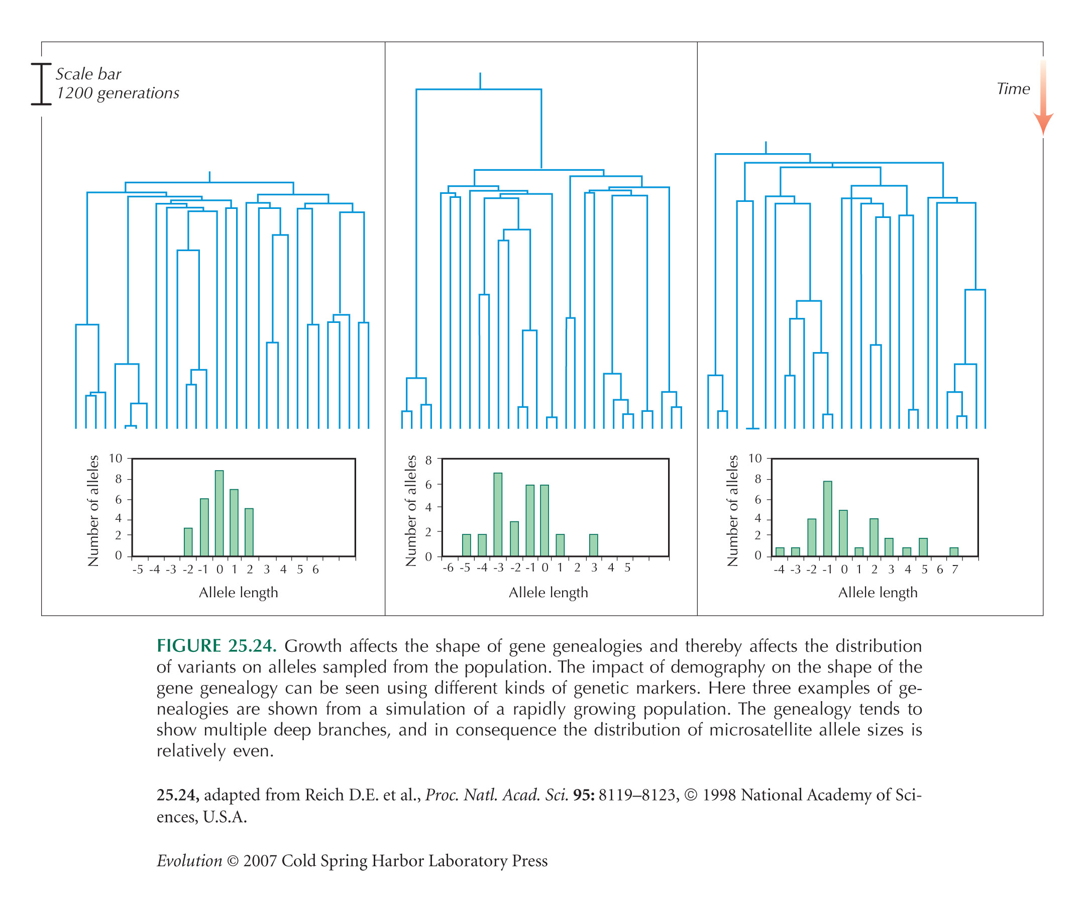
NOTE 15N: This difference in the mismatch distribution has been used as a way to distinguish alternative population histories using mitochondrial DNA. However, in any one realization from a population of constant size, the distribution is dominated by when the oldest pair of lineages coalesce and is highly random. The method is not as accurate as the above comparison of the distribution over many independent realizations (see Fig. P15.6B and Fig. 25.24). Moreover, accuracy is not much improved by taking larger samples: The main randomness is in when the MRCA lived.
NOTE 15O: It is perhaps counterintuitive that two genes that now happen to be sitting together in the same genome are quite likely to be together even very far back in the past, provided 2Ner is not too large.