 |
|
|
|
|
Evolution Chapter 15 Answers
|
Answer 15.1
|
| i) |
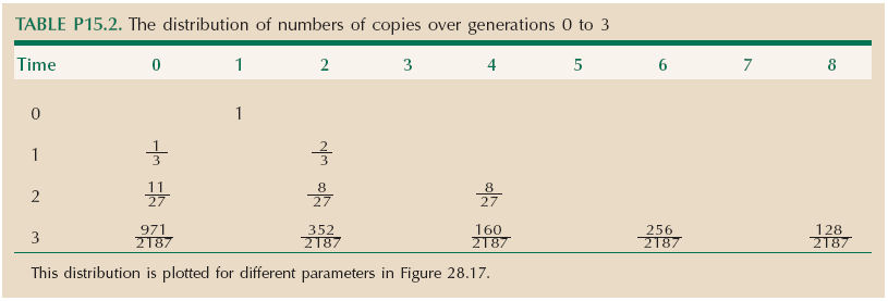
After one generation, there is a 1/3 chance that there are no copies and 2/3 chance that there are two. If there were no copies, then in the second generation, there would still be none. If there are two copies, both may die (chance 1/9), or one may divide and the other may die (chance 2 × 1/3 × 2/3 = 4/9), or both may divide, giving four copies (chance 4/9). The chance of there being no copies is therefore 1/3 + 2/3 × 1/9 = 11/27; the chance that there are two copies is 2/3 × 4/9, and the chance that there are four copies is 2/3 × 4/9. Continuing in this way, we get the probability distribution over time; however, successive generations take more and more calculation. (See Table P15.2.)
|
| ii) |
The expected number of copies increases by 2 × 2/3 = 4/3 in every generation. After ten generations, the expected number is (4/3)10 = 17.76. However, this is an average over a very broad distribution.
|
| iii) |
The probability that the mutant allele will be lost is the chance that it dies before reproducing (1/3) plus the chance that it reproduces (2/3) and that both its offspring leave no descendants (Q2). Thus, Q = 1/3 + (2/3)Q2. This has solution Q = 1/2. (Q = 1 is a trivial solution: If an allele is lost, it stays lost.) (This can be found using the formula for a quadratic equation or by drawing graphs of Q and 1/3 + (2/3)Q2 and finding where they cross.) This derivation is explained in Chapter 28.
|
| iv) |
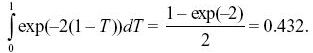
Now, there is probability 0.01 of zero copies, 0.97 of one, and 0.02 of two, after 1 minute. The expected number of copies is 0.97 × 1 + 0.02 × 2 = 1.01, and so after t minutes, the expected number is 1.01t ~ exp(0.01t). (See Fig. P15.2.)
|
| v) |
We now have a recursion Q = 0.01 + 0.97Q + 0.02Q2, which still has solution Q = 1/2. The probability of loss is the same, whether we have reproduction in discrete generations or in continuous time.
|
| vi) |
The overall expectation, exp(0.01t), is the sum of probability Q=1/2 of ultimate loss, times zero, plus probability P = (1 – Q) = 1/2 of not being lost, times the expected number given that the allele is not lost,  , exp(0.01t) = (1/2) × 0 + (1/2) × . Therefore, = exp(0.01t)/(1/2) = 2 exp(0.01t). (This is an application of Bayes’ Theorem; see Box 28.4.) , exp(0.01t) = (1/2) × 0 + (1/2) × . Therefore, = exp(0.01t)/(1/2) = 2 exp(0.01t). (This is an application of Bayes’ Theorem; see Box 28.4.)
|
|
Answer 15.2
|
| i) |
In the first generation, the variance of allele frequency is p0q0/2N = (0.3 × 0.7)/(2 × 20) = 0.00525. The distribution will be approximately normal, with standard deviation  = 0.073. After five generations, the distribution is approximately normal, with variance five times as large (5 × 0.00525 = 0.02625, s.d. 0.162). However, this overlaps the lower boundary at p = 0, and so just assuming that the allele frequencies diffuse outward at a constant rate has become a poor approximation. = 0.073. After five generations, the distribution is approximately normal, with variance five times as large (5 × 0.00525 = 0.02625, s.d. 0.162). However, this overlaps the lower boundary at p = 0, and so just assuming that the allele frequencies diffuse outward at a constant rate has become a poor approximation.
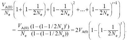
The exact formula for the variance at time t is given in Box 15.1 as p0q0(1 – (1 – 1/2N)t) (i.e., 0.00525, 0.0250, 0.134 at t = 1, 5, 40 generations). At large times, populations fix for either Q or P, ultimately with probability 0.7, 0.3, respectively; allele frequencies in any populations that are not fixed are roughly uniformly distributed. The form of the distribution is shown in Figure 15.3A for a starting frequency of p0 = 0.5; it is shown for the present example in Figure P15.3.
|
| ii) |
We need to find the expected proportion of heterozygotes formed by random mating within a population with allele frequency p, E[2pq]. This is derived in Box 15.1 as 2(p0q0-var(p)) = 2(p0q0(1 –1/2N)t), or 0.420, 0.410, 0.370, 0.153 at t = 0, 1, 5, 40 generations. Because the overall allele frequency over the whole collection of populations stays constant at p0 = 0.3, the heterozygosity of a random offspring with parents from different populations also stays constant at 2p0q0 = 0.42. In this sense, the overall genetic diversity stays constant but shifts from variation within populations to variation between them.
|
|
Answer 15.3
|
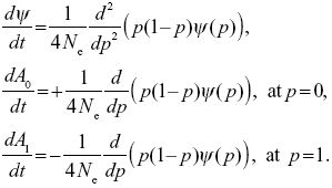
| i) |
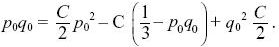
For a neutral allele, the allele frequency stays constant on average (M = 0), and the variance of fluctuations in allele frequency is V = p(1 – p)/2Ne. So, from the equation in Chapter 28:
|
| ii) |
If we substitute ψ = C e–t/2Ne into the first equation, we find that it is a solution.
|
| iii) |
Substituting into the second equation,
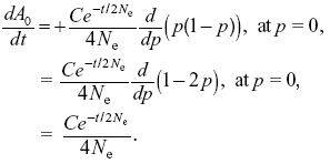
We see that this is satisfied by A0 = C0 – (C/2) exp(–t/2Ne), where C0 is some unknown constant; it can be satisfied similarly for A1.
|
| iv) |
The constraints on the sum, the mean, and the variance are
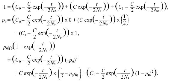
The first two equations lead to C0 = q0, C1 = p0 (i.e., the ultimate probabilities of loss or fixation equal the initial allele frequencies). The last constraint is then
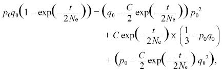
so that
Using q02 + 2p0 q0 + p02 = 1, we find that C = 6p0q0. For example, at t = 4Ne, the chance that a population will still be polymorphic is 6p0q0 exp(–2) ~ 0.17 for p0 = 0.3. NOTE 15B
|
|
Answer 15.4
|
| i) |
The additive genetic variance decreases by a factor (1 – 1/2Ne) per generation (see p. 418). Initially, VA(0) = VE, and so after 30 generations, VA(30) = (1 – 1/2Ne)30, VE = 0.362VE, and the heritability is VA/(VA + VE) = 0.266.
|
| ii) |
Mutation increases additive variance by Vm, whereas drift reduces it by –VA/2Ne. When mutation balances drift, Vm = VA/2Ne, and so VA = 2NeVm. Here, this is 2 × 15 × 0.005Ve = 0.15Ve. The heritability is then h2 = 0.15/1.15 = 0.13. NOTE 15C
|
| iii) |
The variance of the trait mean increases by VA(0)/Ne in the first generation. In the next generation, it increases by a further VA(1)/Ne = (VA(0)/Ne) (1 – 1/2Ne). After t generations it will equal
After 30 generations, the variance in trait mean will be 2VE × 0.362 = 0.724Ve; its s.d. tends to 0.851  ; because VP = 2VE initially, the s.d. of the trait mean equals 0.602 ; because VP = 2VE initially, the s.d. of the trait mean equals 0.602  . In the indefinite future, the variance of the trait mean tends to a maximum of 2VA(0); its s.d. is equal to the initial phenotypic standard deviation. NOTE 15D . In the indefinite future, the variance of the trait mean tends to a maximum of 2VA(0); its s.d. is equal to the initial phenotypic standard deviation. NOTE 15D
|
|
Answer 15.5
|
| i) |
and so
NOTE 15E
Roughly equal amounts of drift occur during the brief bottlenecks as during the longer periods of larger size.
|
| ii) |
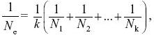
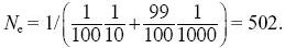
From Box 15.2,
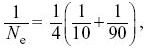
and so Ne = 36.
|
| iii) |
From Box 15.2, 1/Ne = (2 + V)/4N. The mean offspring number is
so that the population is in steady state. The variance of offspring number, V, is

three times the variance of a Poisson distribution with the same mean. Thus, Ne = 4 × 100/(2 + 6) = 50. NOTE 15F
|
|
Answer 15.6
|
| i) |
First, consider the chance that a randomly chosen gene in the daughter is IBD with a random gene in the queen. This is the chance that the daughter’s gene came from the queen times the chance that it was the same gene as we chose from the queen: fQD= 1/4. Now, consider the chance that two genes, one from each daughter, are IBD. This is the chance that they both came from the father (1/4), in which case they must be the same gene, plus the chance that they both came from the queen, times the chance that they are the same gene (1/4 × 1/2 = 1/8). So, fDD = 3/8.
|
| ii) |
If the queen mates with many different males, then if two genes in the daughters both came from the father, they will have come from different fathers and will be unrelated. So, the coefficient of kinship between daughters falls to 1/8, the chance that they both came from the same gene in the queen. (See Fig. P15.4.) NOTE 15G
|
|
Answer 15.7
|
| i) |
We use the formula in Box 15.3 for the probability of identity by descent:
There are two loops, one via the grandfather and one via the grandmother, and each contain six individuals. Measuring the probability of identity relative to the grandparents’ generation, fA = 0 by definition. Thus,
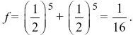
(See Fig. P15.5.)
|
| ii) |
The chance that the offspring is homozygous for the recessive disease allele is the chance that its genes are not IBD times the frequency of homozygotes in a random pair of genes, plus the chance that they are IBD times the chance that the ancestral gene was a disease allele: fp + (1 – f)p2 = 0.00031. This is much higher than with no inbreeding: p2 = 0.000025.
|
| iii) |
Now, we just multiply by (1 + fA) for both of the two loops, with fA = 1/16, giving (17/16)(1/32) + (17/16)(1/32) = 17/256, not much greater. The incidence of the disease is now 0.00036.
|
| iv) |
We need to work out the average IBD between the two genes in a randomly chosen individual. If that individual does not come from an inbred marriage, then they will not be IBD. If it does, they will be IBD with probability f = (1/16)(1 + fA). The overall probability of identity, therefore, is f = (1/10)(1/16)(1 + fA). But, the average probability of identity in the ancestor, fA, must equal the current identity if the population is at steady state. So, f = fA = 1/159. (The correction for inbreeding in the ancestor has made hardly any difference.) The incidence of the disease is fp + (1 – f)p2 as before, which is 0.000056. Roughly equal numbers of cases are from inbred and outbred marriages (the two terms in the expression fp + (1 – f)p2). NOTE 15H
|
|
Answer 15.8
|
| i) |
The expected time back to the MRCA of two lineages is just 2Ne generations.
|
| ii) |
There are three pairs of lineages that might coalesce, so the expected time back to the first coalescence is (2Ne/3) generations. The expected time back to the MRCA of the sample of three is (2 + 2/3)Ne = (8/3)Ne.
|
| iii) |
With five lineages, there are 5 × 4/2 = 10 pairs of lineages, so the expected time is 2Ne(2/(5 × 4)) = 2Ne/10. In total,
NOTE 15I NOTE 15J
|
| iv) |
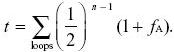
The chance that this new lineage does not coalesce with the five others, during the time T 5 for which they exist, is exp(–5T5/2Ne). Similarly, the chance that it also does not coalesce with four lineages while those four exist is exp(–4T4/2Ne). So, the chance that there is now an older MRCA is the chance that the sixth lineage does not coalesce during T5, T4, T3, or T2: exp(–5T5/2Ne)exp(–4T4/2Ne)exp(–3T3/2Ne)exp(–2T2/2Ne).
A crude approximation is that T5 = 2Ne/10, T4 = 2Ne/6, T3 = 2Ne/3, T2 = 2Ne. This gives exp(–1/2)exp(–2/3)exp(–1)exp(–2) = exp(–4.167) = 0.0155. The exact result uses the fact that the expectation of exp(–aTk/(2Ne), when Tk is exponentially distributed with rate (k(k – 1)/2)/(2Ne), is (k(k – 1)/2)/(a + k(k – 1)/2). Hence, the probability is 1/15 = 0.067. This is somewhat higher, because this calculation has allowed for random variation in the coalescence times.
|
|
Answer 15.9
|
| i) |
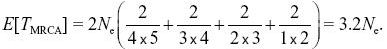
The expected time to coalescence of a randomly chosen pair is 2Ne generations, and so they have had on average 4Ne generations to diverge. Therefore, the probability that two sites differ between the pair is π = 4Ne μ = 0.01.
|
| ii) |
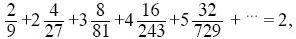
If we assume that every mutation is at a new site (i.e., the infinite sites model), then the expected number of segregating sites is just the number of mutations that have occurred within the genealogy. This is the total length of the genealogy times the total mutation rate, μL, over the length of the sequence, L. Now, we know that the time taken for n lineages to coalesce averages E[Tn] = 2Ne/(n(n – 1)/2) generations, because there are n(n – 1)/2 pairs that can coalesce. The corresponding length of genealogy is nTn. If we add up over the times for which n, n – 1,..., 2 lineages are present and multiply by the mutation rate, we then have
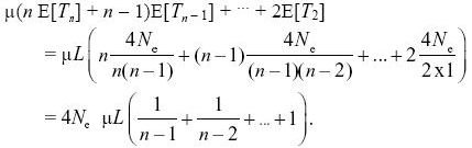
For n = 10, this equals 2.83 × 4Neμ × L = 283 segregating sites. NOTE 15K
|
| iii) |
If all lineages coalesced in a bottleneck T = 106 generations ago, then the pairwise diversity would still be π = 2Tμ = 0.01. The number of segregating sites is the total mutation rate times the length of the genealogy, nT × μL = 500, about twice the expectation for a constant-sized population. This reflects the fact that with a star genealogy, each mutation appears only once and so contributes minimally to pairwise diversity. The expectations become more different for larger samples. With n = 100 genes, for example, we expect 4NeμL(1/99 + 1/98 + ··· + 1) = 518 segregating sites with a constant-sized population but 5000 segregating sites with a star genealogy. NOTE 15L NOTE 15M
|
|
Answer 15.10
|
| i) |
The time, T, to common ancestry of a pair of sequences is exponentially distributed with mean E[T] = 2Ne. The number of differences is Poisson-distributed, with mean 2μLT, where L = 1000. Therefore, the overall mean is 2μLE[T] = 4NeμL = 12. (This is just the length of sequence times the nucleotide diversity, Lπ.) The variance of the number of differences is due to variation in coalescence times (var(2μLT) = (2μL)2var(T) = (2μL)2(2Ne)2 = (4NeμL)2) plus variation in the number of mutations, given T; the latter is Poisson-distributed and has variance equal to its mean, 4NeμL. So, the total variance is 4NeμL+(4NeμL)2 = 12 + 144 = 156; the standard deviation is 12.5, almost all variance is due to variation in coalescence time, rather than the Poisson distribution of number of mutations.
|
| ii) |
If all lineages coalesced 2 × 10⁶ generations back, then pairwise diversity would be the same, but the only variance in number of differences would be due to the Poisson distribution: 4NeμL = 12. (See Fig. P15.6.) NOTE 15N
|
|
Answer 15.11
|
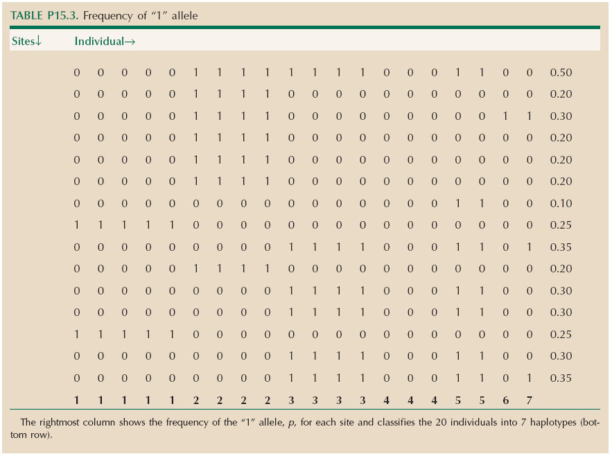
| i) |
Table P15.3 shows the frequency of the “1” allele, p, for each site (right column) and classifies the 20 individuals into 7 haplotypes (bottom row). Summing 2pq across all the sites and then dividing by the length of sequence gives (0.25 + 0.25 + ...)/12000 = 0.00047.
|
| ii) |
There are seven haplotypes. The total number of possibilities is 215 = 32,768. The most common would be expected to be all zeros and to have a frequency among haploid genomes equal to the product of the frequencies of the “0” alleles: (1 – 0.50)(1 – 0.20) … = 0.0084. In fact, this haplotype has frequency 0.10.
|
| iii) |
The numbers of copies of the four possible two-locus genotypes for the first two rows are
Thus, 11 is at frequency 0.2, but would be expected to be at 0.5 × 0.2 = 0.1. Therefore, D is the difference between observed and expected frequencies and equals 0.1. This is the maximum possible D for these allele frequencies, so D/Dmax = 1. The correlation measure is r = 0.5.
For the first and last rows,
Thus, D = 0.3 – 0.35 × 0.5 = 0.125, D′ = 0.125/(0.5 × 0.35) = 0.714, and r = 0.524.
|
| iv) |
Even after simplifying by deleting all rows that are the same and all columns that are the same, the problem still takes some thought:
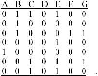
It is impossible to relate these 20 sequences by a genealogy. The easiest way to see this is to look at rows 3 and 6 in the reduced table (bold), which show all four combinations 00, 01, 10, 11. Thus, there is one allele that distinguishes B,F,G from A,C,D,E and another allele that distinguishes A,B,D,F from C,E,G. These groups overlap, which is impossible unless there has been recombination. In general, seeing a pair of sites that show all four possible combinations (i.e., that are not in the maximum possible linkage disequilibrium) excludes a genealogy. (We could have seen this from iii), where the first and last rows were shown to be in less than maximal LD, i.e., showed all four types.)
|
|
Answer 15.12
|
| i) |
The total length of the genealogy is 40,000 generations, and a recombination event anywhere on this ancestry may produce a different genealogy. The rate of such events is 1/40,000, and so the average map distance will be ~0.0025 cM. (Recall that 1 cM corresponds to a recombination rate of 0.01.) More precisely, the map distance will be exponentially distributed with mean 0.0025 cM.
|
| ii) |
The recombination will occur at some time t in the past and is equally likely to be anywhere on either branch. The recombinant lineage will wander back and may coalesce with either of the two branches at a total rate 2/(2Ne). (If it coalesces with the original branch, the common ancestor will be the same, but if it coalesces with the other branch, the common ancestor will be more recent.) The chance that it does not coalesce with either branch during time (20,000 – T) is exp(–(20,000 – T) × 2/(2Ne)), in which case, the common ancestor must be earlier than 20,000 generations. It is convenient to measure time relative to 2Ne =20,000 generations, and so we can define T = t/(20,000). The average of this probability over a uniformly distributed time is then
A rough answer, avoiding integration, would be to just set T to its average, 1/2, giving a probability exp(–1) = 0.367.
|
|
Answer 15.13
As we trace back, lineages on the same genome recombine apart at a rate r = 10–4 per generation (0.01 cM means a recombination rate of 10–4). Conversely, lineages on different genomes coalesce, coming together in a single individual, at a rate 1/2Ne. Suppose that there is a chance x that they are together. They split apart at a rate rx but come together at a net rate (1 – x)/2Ne. At equilibrium, these rates balance, and so rx = (1 – x)/2Ne. Therefore, the chance that they are together in the same genome is x = 1/(1 + 2Ner). In this example, x = 1/3. NOTE 15O
|
References
Clayton G.A. and Robertson A. 1955. Mutation and quantitative variation. Am. Nat. 89: 151–158.
Lynch M. and Hill W.G. 1986. Phenotypic evolution by neutral mutation. Evolution 40: 915–935.
|
|
|
