Chapter 28
Models of Evolution
 Quantitative models play a crucial role in evolutionary biology, especially in population genetics. Mathematical analysis has shown how different evolutionary processes interact, and statistical methods have made it possible to interpret observations and experiments. The availability of computing power and the flood of genomic data have made quantitative methods even more prominent in recent years. Quantitative models play a crucial role in evolutionary biology, especially in population genetics. Mathematical analysis has shown how different evolutionary processes interact, and statistical methods have made it possible to interpret observations and experiments. The availability of computing power and the flood of genomic data have made quantitative methods even more prominent in recent years.
Although we largely avoid explicit mathematics in Evolution, mathematical arguments lie behind much of what is discussed. In this chapter, the basic mathematical methods that are used in evolutionary biology are outlined. The chapters in the book can be understood in a qualitative way without this chapter, and that may be appropriate for an introductory course. Similarly, many of the problems associated with Chapters 13–23 involve only elementary algebra and do not require the mathematical methods explained in this chapter. However, reading through this chapter and working through the problems that depend on it will give you a much stronger grasp of evolutionary modeling and will allow you to fully engage with the most recent research in the field.
Most students will have had some basic courses in statistics, focusing on methods for testing alternative hypotheses and making estimates from the data. Although we do emphasize the evidence that is the basis for our understanding of evolutionary biology, we do not do more than touch on methods for statistical inference. However, our understanding of the evolutionary processes does fundamentally rest on knowledge of probability: Indeed, much of modern probability theory has been motivated by evolutionary problems. This is true both when we follow the proportions of different genotypes within a population and, more obviously, when we follow random evolutionary processes (Chapter 15) in explicitly probabilistic models. (The importance of probability will become apparent when you work through the problems.) In this chapter, we discuss the definitions and meaning of probability and summarize the basic theory of probability.
This chapter begins with an explanation of how mathematical theory can be used to model reproducing populations. Next, we discuss how deterministic processes (i.e., those with no random element) can be modeled by following genotype frequencies. Then, random processes are examined, summarizing important probability distributions and describing two fundamentally random phenomena, branching processes and random walks. The chapter ends with an outline of the diffusion approximation, which has played a key role in the development of the neutral theory of molecular evolution (p. 59).
Throughout this chapter, only straightforward algebra and some basic calculus are used. The emphasis is on graphical techniques rather than manipulation of algebraic symbols. Thus, many of the problems can be worked through using a pencil and graph paper. In general, it is more important to understand the qualitative behavior of a model than to get exact predictions: Indeed, models that are too complex may be as hard to understand as the phenomenon being studied (p. 382). This a particular problem with computer simulations: These can show complex and intriguing behavior, but, all too often, this behavior is left unexplained. This chapter should give you an appreciation of the key role that simple mathematical models play in evolutionary biology.
Mathematical Theory Can Be Used in Two Distinct Ways
To aid in understanding evolutionary biology, mathematical techniques can be used in two ways (Fig. 28.1). The first is to work out the consequences of the various evolutionary processes and to identify the key parameters that underlie evolutionary processes. For example, how do complex traits, which are influenced by many genes, evolve (Chapter 14)? How do random drift, gene flow, and selection change populations (Chapters 15–17)? How do these evolutionary forces interact with each other and with other processes (Chapter 18)? As an aid in answering questions like these, the main role of mathematical theory is to guide our understanding and to develop our intuition rather than to make detailed quantitative predictions. Often, verbal arguments can be clarified using simple “toy models,” which show whether an apparently plausible effect can operate, at least in principle. Much of our progress in understanding sexual selection (Chapter 20) and the evolution of genetic systems (Chapter 23) has come from this interplay between verbal argument and mathematical theory. Thus, although only verbal arguments are presented in other chapters, these correspond to definite mathematical models.
Mathematical techniques can also identify key parameters underlying evolutionary processes. For example, for a wide range of models, the number of individuals that migrate in each generation determines the interaction between random drift and migration. This number of migrants can be written as Nm, where N is the number in the population and m is the proportion of migrants (see Box 16.2). Similarly, the parameter Ns (which is, roughly, the number of selective deaths per generation) determines the relative rates of random drift and selection. Sometimes, mathematical techniques can identify a key quantity that determines the outcome of a complex evolutionary process. For example, the total rate of production of deleterious mutations determines the loss of fitness due to mutation (p. 552), and the inherited variance in fitness determines the overall rate of adaptation (pp. 462 and 547–549). Once these key quantities have been identified, experiments can then be designed that focus on measuring them, and other complications (e.g., numbers of genes and their individual effects) can be ignored.
Mathematical theory is now being used in a second, and quite distinct, way. The deluge of genetic data that has been generated over the past few decades demands quantitative analysis. Thus, recent theory has focused on how to make inferences about evolving populations, based on samples taken from them. Some questions are quite specific: for example, using forensic samples to find the likely ethnic origin of a criminal, finding the age of the mutation responsible for an inherited disease, or mapping past population movements (pp. 434, 743–748, and 768–773). Others are broader: such as finding what fraction of the genome has a function (pp. 542–547) or measuring rates of recombination along chromosomes (Fig. 15.19).
Answering many of these questions requires tracing the ancestry of genes back through time (Fig. 28.1b) rather than modeling the evolution of whole populations forward in time (Fig. 28.1a). Thus, making inferences from genetic data requires new kinds of population genetics and new statistical techniques. These have been especially important in the development of the neutral theory (p. 59) and, more recently, in analyzing DNA sequence data (e.g., pp. 435–437 and 760–765).
Deterministic Processes
A Population Is Described by the Proportions of the Genotypes It Contains
It is populations that evolve and it is populations that we must model. Populations are collections of entities that can be of several alternative types; thus, it is necessary to follow the proportions of these different types. For example, when dealing with a collection of diploid individuals, and focusing on variation at a single gene with two alleles, the proportions of the three possible diploid genotypes QQ, PQ, and PP must be followed. If, instead, the focus is on the collection of genes, then the frequencies of the two types of gene (labeled, for example, Q and P) are followed.
Before going on, two points need to be made concerning terminology. First, different kinds of gene are referred to as alleles. Thus, the proportions of alleles Q and P can be written as q and p, which are known as allele frequencies, and, clearly, q + p = 1. (Genetic terminology is discussed in more detail in Box 13.1.) Second, perhaps the most important step in building a model is to decide which variables describe the population under study. When a population is modeled, these variables are either the allele frequencies or the genotype frequencies of the different types or genealogies that describe the ancestry of samples of genes. Variables must be distinguished from parameters, which are quantities that determine how the population will evolve, such as selection coefficients, recombination rates, and mutation rates. As a population evolves, the parameters stay fixed, but the variables change.
Physics and chemistry also deal with populations, but these populations are atoms and molecules instead of genes and individuals. However, atoms are conserved intact, and although molecules may be transformed by chemical reactions, their constituent atoms are not affected (Fig. 28.2A). In biology, the situation is fundamentally different: individuals, and the genes they carry, die and reproduce. This leads to more complex—but also more interesting—phenomena.
In the simplest case, offspring are identical to their parents (Fig. 28.2B). In ecological models, the assumption is that females of each species produce daughters of the same species, and so the numbers of each species in the whole ecosystem are followed. (Often, males have a negligible effect on population size and so can be ignored.) The same applies to asexual populations (e.g., bacteria), where offspring are genetically identical to their parents, or where the different alleles of a single gene are followed (Fig. 28.2B). Even in this simplest case, however, the reproduction of each individual is affected by the other individuals in the population, leading to a rich variety of phenomena (pp. 470–472 and 505–508). Different species or different asexual genotypes compete with each other, and the different alleles at a single genetic locus combine to form different diploid genotypes.
Sexual reproduction is harder to model, because two individuals come together to produce each offspring, which differs from either parent (Fig. 28.2C). We can no longer follow individual genes but must instead keep track of the proportions of all the different combinations of alleles that each individual carries. Although each gene stays intact per se, the set of genes that it is associated with changes from generation to generation.
Whether reproduction is sexual or asexual, a population can be modeled by keeping track of the proportion of each type of offspring. This is much harder for a sexual population, because so many different types can be produced by recombination (Fig. 28.3). However, the basic approach to modeling is the same as when there are just two types. In this chapter, we will work through the simplest case, that of two alleles of a single gene. The basic principles generalize to more complicated cases, where a large number of types must be followed (see Problem 19.15 and Problem 23.7).
Reproducing Populations Tend to Grow Exponentially
Evolution usually occurs so slowly that it can be treated as occurring continuously through time, as a continuous change in genotype frequencies or in the distribution of a quantitative trait. Sometimes, evolution may be truly continuous. For example, suppose that in each small time interval, organisms have a constant chance of dying and a constant chance of giving birth, regardless of age. Then, only their numbers through time, n(t), need to be followed. Their rate of increase—that is, the slope of the graph of numbers against time—is written as

This is a simple differential equation that gives the rate of change of the population size in terms of its current numbers. The solution to this equation can be seen in qualitative terms from the graph of Figure 28.4, for r = 1. When numbers are small, the rate of increase is small, but as numbers increase, so does the rate, giving the characteristic pattern of exponential change. This solution is written as
n(t) = n(0) ert or n(0) exp(rt),
where e = 2.71827... . This pattern can also be thought of as an approximation to a discrete model of geometric growth, in which numbers increase by a factor (1 + r) in every time unit. After t generations, the population has increased by a factor (1 + r)t, which tends to exp(rt) for small r. (For example, 1.110 = 2.594, and 1.01100 = 2.705, approaching e = 2.718... .)
The exponential relationship often needs to be inverted, in order to find the time taken for the population to grow by some factor (Fig. 28.5). This inverse relationship is the natural logarithm, defined by log(exp(x)) = x. Thus,
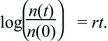
Using this formula, the time it takes for a population to grow by a factor e = 2.718 is given by rt = log(e) = 1, which is a time t = 1/r. Similarly, it takes a time log(10)/r ~ 2.30/r to increase tenfold, and twice that to increase 100-fold (log(100)/r ~ 4.60/r). (In this book, natural logarithms are always written as log(x). They can be written as loge(x) or ln(x) to distinguish them from logarithms to the base 10, log10(x), which were commonly used for arithmetical calculations. Now that electronic calculators are so widespread, logarithms to the base 10 are rarely seen.)
If a population contains two types, Q and P, each with its own characteristic growth rate rQ and rP, then the numbers of each type will grow exponentially. As explained in Box 28.1, the proportions change according to

where the selection coefficient s is the difference in growth rates, rP – rQ. (The consequences of this formula were explored in detail in Box 17.1.) Thus, in continuous time, the appropriate measure of fitness is the growth rate r, and the selection coefficient is the difference in fitness between genotypes. In any actual population, growth rates will change over time. If the population is to remain more or less stable, growth rates must decrease as the population grows and increase as the population shrinks. However, provided that the growth rates of each genotype change in the same way, the differences between them stay the same, and so changes in allele frequency are not affected by changes in population size (Fig. 28.6).
Box 28.1 Selection in Discrete and Continuous Time
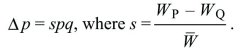
Whether a population reproduces in discrete generations or continuously through time, the rate of change in allele frequency is Δp = spq, where s is the selection coefficient, which is the difference between the relative fitnesses of the two alleles.
Discrete Time: Imagine a haploid population, with alleles Q, P at frequencies q, p (where q + p = 1). Each gene of type Q produces WQ copies, and each gene of type P produces WP. In the next generation, the numbers of each will be in the ratios qWQ:pWP. Dividing by the total gives the new frequencies:
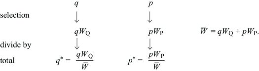
The change in allele frequency is

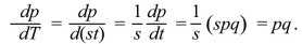
This can be written as
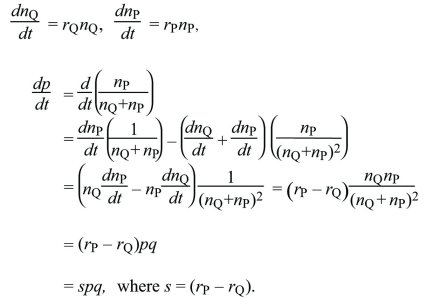
Continuous time: Suppose that for types Q, P, their numbers nQ, nP are each growing exponentially at rates rQ, rP. How does the allele frequency, p = nP/(nQ + nP) change? This is found by differentiating with respect to t and applying the rules for differentiating products and ratios:
Gradual Evolution Can Be Described by Differential Equations
The basic differential equation dn/dt = rn has been presented as an exact model of a homogeneous population that reproduces continuously in time. However, it is also a close approximation to populations that reproduce in discrete generations, as long as selection is not too strong. The change in allele frequency from one generation to the next is Δp = spq, where the selection coefficient s is again the difference in relative fitness between the two alleles (Box 28.1). Approximating this discrete process as a continuous change in allele frequency p(t) can be thought of as drawing a smooth curve though a series of straight-line segments (Fig. 28.7). More complicated situations are described in Chapter 17; for example, populations may contain a mixture of ages, each with different birth and death rates. However, as long as change is gradual, the population will settle into a pattern of steady growth that can be modeled by a simple differential equation (Box 17.1). It is almost always more convenient to work with differential equations than with discrete recursions, and so most population genetics theory is based on differential equations. Box 28.2 shows how equations can be integrated to find out how long it takes for selection to change allele frequency. Problem 17.9 shows how this method can be used for a variety of models.
Box 28.2 Solving Differential Equations
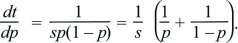
Differential equations such as dp/dt = spq can be solved by thinking of time as depending on allele frequency, t(p), rather than of allele frequency as a function of time, p(t). In other words, we can ask how long it takes a population to go from one allele frequency to another. This is written as
Using the fundamental relation between differentiation and integration,
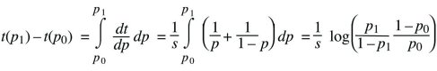
This gives the time taken for the allele frequency to change from p0 to p1. As emphasized in the main text, this time is inversely proportional to the selection coefficient.
This derivation can be seen graphically with the aid of Figure 28.8, which plots s(dt/dp) = 1/pq, the rate of increase of time against allele frequency. The area under the curve is the total time elapsed, T = st. By definition, this equals the integral of 1/pq, which is plotted in Figure 28.9; the gradient of this graph equals 1/pq. This graph gives the (scaled) time that has elapsed. Turning this graph around gives the more familiar graph of allele frequency against time, p(T).
Describing gradual evolution by differential equations can be extended to more complicated situations involving several variables, such as following the frequencies of three or more alleles of one gene or following allele frequencies at multiple genes. In such cases, a set of coupled differential equations are generated, in which the rate of change of each variable depends on all the others:
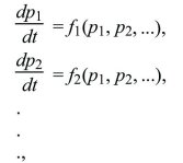
where f1, f2 represent some arbitrary relationship between the present state of the population (described by p1, p2, ...) and its rate of change. Even quite simple systems of this sort can show surprisingly complex behavior, including steady limit cycles or chaotic fluctuations.
The most important point to take from this section is a qualitative one: The timescale of evolutionary change is inversely proportional to the selection coefficient s. In the simplest case, where dp/dt = spq and s is a constant, a new measure of time, T = st, can be defined. Then,
The allele frequency depends only on T; thus, the same equation applies for any strength of selection provided that the timescale is adjusted accordingly.
This can also be done in the more general case, where there is a set of equations with rates all proportional to some coefficient s (dp1/dt = sf1, dp2/dt = sf2, ..., so that dp1/dT = f1, dp2/dT = f2, ...). Thus, all that matters is the scaled time T. For example, the pattern of change would look the same if the strength of selection were halved throughout but would be stretched over a timescale twice as long. Elsewhere in the book, when processes such as migration, mutation, and recombination are considered, we see that change occurs over a timescale set by the rates of the processes involved, and that the pattern itself only depends on the ratios between the rates of the different processes.
Populations Tend to Evolve toward Stable Equilibria
It is hardly ever possible to find an exact solution to the differential equations that arise in evolutionary models. Today, it is straightforward to solve differential equations using a computer, provided that numerical values for the parameters are chosen. However, this is insufficient to understand the system fully, because often there will be too many parameters to explore the full range of behaviors. In any case, the goal usually is to do more than just make numerical predictions. We want to understand which processes dominate the outcome: Which terms matter? How do they interact? What is their biological significance? In this section, we will see how we set about understanding models in this way.
The first step is to identify which parameter combinations matter. For example, we have just seen that, in models of selection, only the scaled time T = st matters, not s or t separately. Often, this can drastically reduce the number of parameters that need to be explored. The next step is to identify equilibria—points where the population will remain—and find whether they are locally stable. In other words, if the population is perturbed slightly away from an equilibrium, will it move farther away or converge back to the equilibrium? There may be several stable equilibria, however, so where the population ends up depends on where it starts. In that case, each stable equilibrium is said to have a domain of attraction (Fig. 28.10A). Conversely, there may be no stable equilibrium, so that the population will never be at rest (Fig. 28.10B). However, identifying the equilibria and their stability takes us a long way toward understanding the full dynamics of the population.
In population genetics, in the absence of mutation or immigration, no new alleles can be introduced. In that case, there will always be equilibria at which just one of the possible alleles makes up the entire population. At such an equilibrium, the allele is said to be fixed in the population. The crucial question, then, is whether the population is stable toward invasion from new alleles. This depends on whether the new allele tends to increase from a low frequency, which it will do if it has higher fitness than the resident allele. Thus, analysis is especially simple if, most of the time, the population is fixed for a single genotype. In that case, the fate of each new mutation is examined to determine whether the mutation can invade to replace the previous allele.
Matters are more complicated if, when an allele invades, it sets up a stable polymorphism with the resident allele. Whether new alleles can invade this polymorphic state can still be determined, because such invasion depends only on whether or not a new allele has higher fitness than that of the residents. A substantial body of theory, known as adaptive dynamics, is used to analyze situations like this by making the additional assumption that invading alleles are similar to the resident (Fig. 28.11). This approach is best thought of as a way of exploring the dynamics when a range of alleles is available rather than as an actual model of evolution. (For one thing, when new alleles are similar in fitness to the residents, evolution will be very slow [Fig. 28.11].) In Chapter 20, we looked at other ways of finding what kinds of phenotypes will evolve. In particular, evolutionary game theory focuses on whether a resident phenotype is stable toward invasion by alternatives. Here, the analysis avoids making assumptions about the genetics by simply comparing the fitnesses of different phenotypes. All of these methods are guides to the direction of evolution rather than ways of making exact predictions.
Stability Is Determined by the Leading Eigenvalue
How do we find the stability of a polymorphic equilibrium in which two alleles coexist? The simplest example is that of a single diploid gene, where the heterozygote is fitter than either homozygote. If, for example, the fitnesses of QQ, PQ, PP are 1:1+s:1, then the allele that is less common finds itself in heterozygotes more often and so tends to increase. In Box 17.1, it was shown that
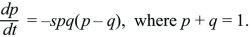
There are equilibria where an allele is fixed (p = 0, 1). To see whether the equilibrium at p = 0 is stable toward the introduction of an allele, assume that p is very small, so that q is close to 1. Then, dp/dt ~ +sp, and a rare P allele will increase exponentially at a rate s (i.e., p(t) = p(0)exp(st), for p << 1). Similarly, a rare Q allele will increase as exp(st). There is also a polymorphic equilibrium where p = q = ½, so that p – q = 0. To show that this is stable, suppose that allele frequency is perturbed slightly to p = ½ + ε, where ε is very small. Then,
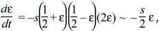
where we have ignored small terms such as ε2. Perturbations will decrease exponentially at a rate –s/2, so that ε(t) = ε(0)exp(–st/2). The polymorphism is, therefore, stable. Equations such as this, in which the variables change at rates proportional to their values, are termed linear. Because they do not include more complicated functions (such as ε2 or exp(ε)), they behave much more simply than the nonlinear equations that describe the full dynamics (here dp/dt = –spq(p – q)).
In this simple, one-variable example, it can be easily seen, without going through the stability analysis, that a polymorphism must be stable (Fig. 28.12). With more variables, however, the outcome is not at all obvious, and a formal stability analysis becomes essential.
There are three key points (which also apply with slight modification in more complex situations) to take from this first example.
-
When near to an equilibrium, the equations almost always simplify to a linear form: dε/dt = λε. The rate of change, λ, is known as the eigenvalue.
-
Therefore, perturbations increase or decrease exponentially, as exp(λt).
-
Equilibria are unstable if λ > 0, so that perturbations grow, and are stable if λ < 0.
We now show how these points extend to an example involving two variables.
Stability Analysis Extends to Several Variables
Suppose that there are two subpopulations, which exchange a proportion m of their genes per unit time. (Such subpopulations are referred to as demes; see p. 441.) An allele is favored in one deme by selection of strength s but reduces fitness by the same amount in the other deme. The entire system is described by two variables—namely, the allele frequencies in the two demes, p1, p2. In Box 28.3, it is shown that there are two equilibria at which one or the other allele is fixed throughout the whole population, and one equilibrium at which both demes are polymorphic. At each equilibrium, a pair of linear equations can be written that describes slight perturbations to the allele frequencies ε1, ε2. Solutions are sought in which these perturbations grow or shrink steadily but stay in the same ratio (e.g., ε1 = e1exp(λt) and ε2 = e2exp(λt)). With two variables, there are two solutions of this form, with two values of λ. Crucially, any perturbation can be written as a mixture of these two characteristic solutions. In the long run, whichever solution grows fastest (or decays the slowest) will dominate. This is just the solution with the largest value of λ, which is known as the leading eigenvalue. This characteristic behavior can be seen in Figure 28.13.
Box 28.3 Migration and Selection in Two Demes
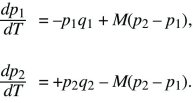
Two subpopulations (or demes) exchange migrants at a rate m per unit time. In deme 1, allele P is disadvantageous, with selection coefficient –s, and in deme 2, allele P is favorable, with selection +s (Fig. 28.14). The allele frequencies p1, p2 change at rates
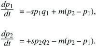
These equations are an exact description of a haploid population reproducing continuously in time but are also a good approximation to a variety of discrete time models of diploids (see Box 16.1).
The problem can be simplified by dividing both sides by s, and scaling time as T = st. Then, it is evident that the solution depends only on the ratio between migration and selection, M = m/s:
Clearly, there are equilibria where only one allele is present (i.e., p1 = p2 = 0 or p1 = p2 = 1). There is also always a polymorphic equilibrium in which selection balances migration. Specifically, selection tends to fix allele Q in deme 1 and P in deme 2, whereas migration tends to make the allele frequencies equal (Fig. 28.13). By symmetry, at this equilibrium, q2 = p1. (In other words, the equilibrium must lie on the diagonal running from upper left to lower right in Fig. 28.13, indicated by a dotted line.) Setting the two equations to 0 and solving reveals that the polymorphic equilibrium occurs where p1q1 = M(p2 – p1) = M(q1 – p1). This can be solved graphically (Fig. 28.15) or algebraically as
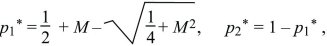
where p1* and p2* are the equilibrium allele frequencies. Only the symmetric model, in which the selection coefficients in each deme are equal and opposite, is analyzed here. If they are different, and if migration is fast enough relative to selection, then whichever allele is favored overall will fix everywhere. However, if the selection coefficients are precisely opposite as above, there will be a polymorphic equilibrium even when migration is fast.
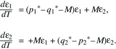
To find the stability of the three equilibria, first suppose that p1 and p2 are small (lower left in Fig. 28.11). The equations then simplify to
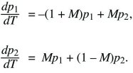
We look for a solution that grows or shrinks steadily, so that p1 = e1exp(λT), p2 = e2exp(λT). Because dp1/dT = λe1exp(λT), and similarly for p2, the factors of exp(λT) cancel throughout and
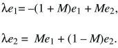
There are two possible solutions: λ = –M ±  . The larger of these must be positive, because > M. So, this equilibrium is unstable, because allele P can invade at a rate λ = –M + > 0. (The green arrow at the bottom left of Figure 28.13 shows this characteristic solution.) The allele invades deme 2 faster than it invades deme 1, because it is favored there; thus, the arrow points upward. A similar argument shows that the equilibrium with P fixed is unstable to invasion by Q (upper right in Fig. 28.13). . The larger of these must be positive, because > M. So, this equilibrium is unstable, because allele P can invade at a rate λ = –M + > 0. (The green arrow at the bottom left of Figure 28.13 shows this characteristic solution.) The allele invades deme 2 faster than it invades deme 1, because it is favored there; thus, the arrow points upward. A similar argument shows that the equilibrium with P fixed is unstable to invasion by Q (upper right in Fig. 28.13).
The polymorphic equilibrium can be analyzed in a similar way, by letting ε1 = p1 – p1* and ε2 = p2 – p2* be small deviations from equilibrium. Discarding small terms such as ε2 and ε3 gives
By searching for solutions of the forms p1 = e1exp(λT) and p2 = e2exp(λT), again an equation for λ is obtained, which has two solutions. The larger is λ = –s(q1* – p1*); because q1* > p1*, the polymorphic equilibrium is stable. As they converge toward this stable equilibrium at a rate λ, populations tend to follow this solution (the leading eigenvector), as indicated by the pair of green arrows in Figure 28.13 (upper left).
The patterns seen in this example of migration and selection in two demes do not quite exhaust the possibilities. Sometimes, no solution of the form ε1 = e1exp(λt) can be found. In such cases, solutions have the form ε1 = e1exp(λt)sin(ωt + θ1), which correspond to oscillations with frequency ω and grow or shrink at a rate λ. The larger value of λ still dominates, because it grows faster, and so the stability of the equilibrium is still determined by whether the larger λ is positive or negative. Even when the model as a whole involves complicated nonlinear interactions, near to its equilibrium it behaves in an approximately linear way. Thus, the standard linear analysis of the behavior near to equilibria tells us a lot about the overall behavior.
Random Processes
Our Understanding of Random Events Is Relatively Recent
Most mathematics is long established. The fundamentals of geometry were worked out at least three millennia ago by the Babylonians, for practical surveying. The Greeks developed both geometry and logic into a rigorous formal system by around 500 B.C. Algebra, the representation of numbers by symbols, was established by Arab mathematicians during the 9th and 10th centuries A.D., and calculus was discovered independently by Gottfried Leibniz and Isaac Newton in the mid-17th century. Yet, the most elementary notions of probability were established much more recently. Probability is a subtle concept; it can be interpreted in a variety of ways and is generally less well understood than most of the mathematics in common use. Some key ideas in basic probability are summarized in Box 28.4.
Box 28.4 Basic Probability
Notation
| | Prob(A), Prob(B) | | probability of events A, B. |
| | fi | | probability that i = 0, 1, 2, ... . |
| | f(x) | | probability density of a continuous variable x. |
Probabilities sum to 1
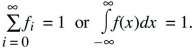
Probabilities of exclusive events sum
Prob(A or B) = Prob(A) + Prob(B) if A and B cannot both occur.
Probabilities of independent events multiply
Prob(A and B) = Prob(A)Prob(B) if the chance of A occurring is independent of whether B occurs, and vice versa.
Expectation
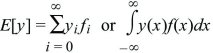
is the expected value of y; it is an average over the probability distribution f.
Mean and variance
The mean of y is E[y], sometimes written  . .
The variance of y is E[(y – )2] or var(y).
The standard deviation of y is  . .
Probability did not become an integral part of physics until the 1890s, when Ludwig Boltzmann showed how gross thermodynamic properties such as temperature and entropy could be explained in terms of the statistical behavior of large populations of molecules. Even then, random fluctuations themselves were not analyzed until 1905, when Albert Einstein showed that Brownian motion, which is the random movement of small particles, is due to collisions with small numbers of molecules (Fig. 28.16).
Arguably, most developments in probability and statistics have been driven by biological—especially, genetic—problems. Francis Galton introduced the ideas of regression and correlation in order to understand inheritance, and Karl Pearson developed these as a tool for analysis of quantitative variation and natural selection (p. 21). The analysis of variance—key to separating and quantifying the causes of variation—was first used by R.A. Fisher in 1918 to describe the genetic variation that affects quantitative traits (p. 393).
Even today, new concepts in probability theory, and new statistical methods, have been stimulated by biological problems. These include Motoo Kimura’s use of the diffusion approximation in his neutral theory of molecular evolution (pp. 59–60 and 425–427). More recently, coalescent models have provided us with a different way of describing the same process of neutral diffusion (pp. 421–425), in terms of the ancestry of genetic lineages. The fundamental importance of random processes in evolution was explained in Chapter 15, and examples of inference from genetic data are given in Chapter 19. Here, basic concepts of probability are reviewed, and some important random processes are described.
A Random Process Is Described by Its Probability Distribution
A probability distribution lists the chance of every possible outcome. These may be discrete (e.g., numbers of mutations), or there may be a continuous range of possibilities (e.g., allele frequencies lying between 0 and 1). For a discrete probability distribution, the total must sum to 1. For a continuous distribution f(x), the chance of any particular value is infinitesimal, but the area under the curve gives the probability that the outcome will lie within some range (Fig. 28.17). Using the notation of integral calculus,

is the chance that x will lie between a and b.
The distribution of a continuous variable is sometimes called a probability density. Again, the total area must sum to 1; that is,

(Fig. 28.17).
The overall location of a distribution can be described by its mean. This is simply the average value of the random variable x, which is sometimes written as  and sometimes as the expectation, E[x] (see Box 28.4). The spread of the distribution is described by the variance, which is the average of squared deviations from the mean (var(x) = E[(x – )2]). The variance has units of the square of the variable (e.g., meters2 if x is a length). Thus, the spread around the mean is often expressed in terms of the standard deviation, equal to the square root of the variance, and with the same units as the variable itself. and sometimes as the expectation, E[x] (see Box 28.4). The spread of the distribution is described by the variance, which is the average of squared deviations from the mean (var(x) = E[(x – )2]). The variance has units of the square of the variable (e.g., meters2 if x is a length). Thus, the spread around the mean is often expressed in terms of the standard deviation, equal to the square root of the variance, and with the same units as the variable itself.
Discrete Distributions
Box 28.5 summarizes the properties of the most important distributions. The simplest cases have only two possible outcomes, such as a coin toss giving heads or tails or one of two alleles being passed on at meiosis. This distribution has often been used when looking at the chance of either of two alleles being sampled from a population, with probability q or p. If the two outcomes score as 0 or 1, then the mean score is p, and the variance in score is pq.
Box 28.5 Common Probability Distributions
Table 28.1 defines commonly used probability distributions. The parameters used in the plots on the right-hand column of the table are two-valued, p = 0.7; binomial, n = 10, p = 0.3; Poisson, λ = 4; exponential, λ = 1; normal, = 0, σ2 = 1; chi-square, n = 10; and Gamma: β = 1, α = 0.5 (red), α = 2 (blue). The factorial 1 × 2 × 3 × ... × n is written as n!. Γ(x) is the gamma function; Γ(n + 1) = n!. Note that the chi-square distribution is a special case of the Gamma distribution.
A natural extension of this two-valued distribution is the binomial distribution. This gives the distribution of the number of copies of one type out of a total of n sampled items. It is the distribution of the sum of a series of independent draws from the two-valued distribution, each with probabilities q, p. (This is the basis of the Wright–Fisher model; see p. 416.) It must be assumed that either the population is very large or each sampled gene is put back before the next draw (“sampling with replacement”). Otherwise, successive draws would not be independent (sampling a P would make sampling more Ps less likely). The mean and variance of a sum of independent events are just the sums of the means and variances of the component means and variances. Therefore, a binomial distribution has mean and variance n times those of the two-valued distribution just discussed, np and npq, respectively. The typical deviation from the mean (measured by the standard deviation) is  , which increases more slowly than n. Therefore, the binomial distribution clusters more closely around the mean as the numbers sampled (n) increase. The binomial distribution approaches a normal distribution with mean np and variance npq as n gets large. , which increases more slowly than n. Therefore, the binomial distribution clusters more closely around the mean as the numbers sampled (n) increase. The binomial distribution approaches a normal distribution with mean np and variance npq as n gets large.
The Poisson distribution gives the number of events when there are a very large number of opportunities for events, but each is individually rare. The classic example is the number of Prussian officers killed each year by horse kicks, described by Ladislaus Bortkiewicz in his 1898 book The Law of Small Numbers. Over the course of 20 years, Bortkiewicz collected data on deaths from horse kicks occurring in 14 army corps and found that the overall distribution of the deaths followed a Poisson distribution. Another example of the Poisson distribution is the number of radioactive decays per unit time from a mass containing very many atoms, each with a very small chance of decaying. For example, a microgram of radium 226 contains 2.6 × 10¹⁵ atoms and is expected to produce 37,000 decays every second; the actual number follows a Poisson distribution with this expectation. Similarly, the number of mutations per genome per generation follows a Poisson distribution, because it is the aggregate of mutations that may occur at a very large number of bases, each with a very low probability (p. 531). The Poisson distribution is the limit of a binomial distribution when n is very large and p is very small. It has mean np = λ, and the variance is equal to this mean (because npq ~ np = λ when p is small). Like the binomial, it converges to a Gaussian distribution when λ is large. We very often need to know the chance that no events will occur. Under a binomial distribution, this is (1 – p)n. As n becomes large, this tends to exp(–np) = exp(–λ), which is the probability of no events occurring under a Poisson distribution. For example, the chance that there are no mutations in a genome when the expected number of mutations is λ = 5 is exp(–5) ~ 0.0067.
Continuous Distributions
We turn now to distributions of continuous variables. The time between independent events, such as radioactive decays or the time between mutations in a genetic lineage, follows an exponential distribution (Fig. 28.18). This distribution has the special property that the expected time to the next event is the same, regardless of when the previous event occurred. (This follows from the assumption that events occur independently of each other.) The exponential distribution has a very wide range; specifically, 1% of the time, events occur closer together than 1% of the average interval, and 1% of the time, they take more than 4.6 times the average. This distribution is closely related to a Poisson distribution. If the rate of independent events is µ, the number within a total time t is Poisson distributed with mean µt.
In contrast, a normal or Gaussian distribution is tightly clustered around the mean. (There is a less than 4.6% chance of deviating by more than 2 s.d., less than 0.27% of deviating by more than 3 s.d., less than 6.4 × 10⁻⁵ of deviating by more than 4 s.d., and so on.) We saw in Figure 14.2 that many biological traits follow a normal distribution. Later in this chapter, we will see why this distribution appears so often. A closely related distribution is the chi-square distribution, which is the distribution of the sum of a number n of squared Gaussian variables, 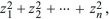 and is written as and is written as  . This determines the distribution of the variance of a sample of n values. . This determines the distribution of the variance of a sample of n values.
There are many other continuous distributions. One that appears quite often is the Gamma distribution, which has two parameters (α, β). It is useful in modeling because it gives a way of varying the distribution from a tight cluster (α large) to a broad spread (α small). The time taken for k independent events to occur, each with rate µ, is gamma distributed, with parameters α = k, β = 1/µ.
Only distributions of a single variable (either discrete or continuous) have been discussed. But distributions of multiple variables will also be encountered, which may be correlated with each other, for example, the distribution of age and body weight. The most important distribution here is the multivariate Gaussian, which has the useful property that the distribution of each variable considered separately, and of any linear combination of variables (e.g., 2z1+3z2, say), is also Gaussian (Box 28.5). This distribution is especially important for describing variation in quantitative traits (pp. 386–387).
Probability Can Be Thought of in Several Ways
We have explained how probabilities can be described and manipulated. But what exactly is a “probability”? The simplest case is when outcomes are equally probable. For example, the chance that a fair coin will land heads up or tails up is always 1/2, and the chance that a fair die will land on any of its six faces is 1/6. Probability calculations often rest on this simple appeal to symmetry. For example, a fair meiosis is similar to a fair coin toss, with each gene having the same chance of being passed on; and if the total mutation rate is 1 per genome per generation, then the probability of mutation is 1/(3 × 109) per generation at each of 3 × 10⁹ bases. However, matters are rarely so simple: Meiotic transmission can be distorted (pp. 587–589), and mutation rates vary along the genome (p. 347). Often, we would like to talk about the probability of events that are not part of any set of symmetric possibilities. What is the chance that the average July temperature will be hotter than 20°C? What are the chances that some particular species will go extinct? What is the chance that some particular disease allele will spread?
One possibility is to define probability as the frequency of an event in a long series of trials or among a set of replicates carried out under identical conditions. This is clear enough if we think of a coin toss or meiotic segregation, because we could imagine repeating the random event any number of times, under identical conditions. However, this is rarely possible in practice (or even in principle). To find the distribution of July temperatures, we could record temperatures over a long series of summers, although there might be good reason to think that the conditions under which the readings were taken are not equivalent, because, for example, the Earth’s orbit, Sun’s brightness, and atmospheric composition fluctuate systematically. The goal is to use this information to find the probability distribution of temperature in one particular summer. Similarly, to answer the other two questions, it is necessary to know the probability of survival of some particular species or allele, which may not be equivalent to any others.
Another problem with using the long-run frequency to define probability is that, given some particular sequence of events, a way to judge the plausibility of the hypothesis is needed. For example, if the sequence is 480 heads and 520 tails, we still need to be certain that the coin is fair (i.e., that the probability of heads = 1/2). There are other possibilities: for example, the probability of heads might be 0.48, or the frequency of heads might increase over the course of the sequence. In real-life situations, we are frequently faced with distinguishing alternative hypotheses on the basis of only one set of data. Invoking hypothetical replicates does not avoid the difficulty, because judgments must still be made on the basis of a finite (albeit larger) dataset.
An apparently quite different view is that probability expresses our degree of belief. This allows us to talk about probabilities not only of events but also of hypotheses. For example, what is the probability that there is life on Mars, or that introns evolved from transposable elements? It is hardly practical to define probability as a psychological measure of actual degree of belief, because that would vary from person to person and from time to time. Instead, probability is seen as the “rational degree of belief” and can be defined as the odds that a rational person would use to place a bet, so as to maximize his or her expected winnings. But put this way, it is either equivalent to the definition based on long-run frequency just discussed (because the expected winnings depend on the long-run frequency) or it is still subjective (because it depends on the information available to each person). These different interpretations of probability influence the way statistical inferences are made.
We (i.e., the authors) favor the view that probability is an objective property, which can be associated with unique events. We calculate probabilities from models. For example, a model of population growth that includes random reproduction gives us a probability of extinction. A model of the oceans and atmosphere gives us the probability distribution of temperature or rainfall in the future. With this view, what is crucial is how hypotheses are distinguished from one another—that is, distinguishing between different models that predict our observations with different probabilities. This issue is explored in more depth in the Web Notes. We take the view that the simplest approach is to prefer hypotheses that predict the actual observations with the highest probability.
Probabilities Can Be Assigned to Unique Events
To give a concrete example of the types of probability arguments that arise in practice, we take as an example predictions of the effects of climate change on specific events. The summer of 2003 was exceptionally hot across the Northern Hemisphere and especially so in Western Europe (Fig. 28.19A). As a result, an additional 22,000–35,000 people died during August 2003, a figure estimated from a sharp peak in mortality rates (Fig. 28.19B); around Paris, there was a major crisis as mortuaries overflowed. In addition, considerable economic damage resulted from crop failures and water shortages. Now, climate is highly variable, and we cannot attribute this particular event to the general increase in global temperatures over the past century, and nor can we say with certainty that it was caused by the greenhouse gases produced by human activities that are largely responsible for that trend. However, we can make fairly precise statements about the probability that such high temperatures would occur under various scenarios.
Models of ocean and atmosphere can be validated against past climate records, so that a narrow range of models is consistent with physical principles and with actual climate. These models predict a distribution of summer temperatures. The summer of 2003 was unlikely, but not exceptionally so. Given current rates of global warming, such hot summers will become common by about 2050. As the distribution shifts toward higher average temperatures, and its variability increases, the chances of extreme events greatly increase (Fig. 28.19C,D). The climate models can be run without including the influence of greenhouse gases and show that the probability of extremely high temperatures would then be much lower. Overall, about half the risk of a summer as extreme as that of 2003 can be attributed to human pollution. It is calculations such as these—estimating the probability of unique events—that lay the legal basis for the responsibility of individual polluters. The point here is that we can and do deal with the probabilities of single, unique events.
The Increase of Independently Reproducing Individuals Is a Branching Process
This chapter is concerned with models of reproducing populations. The simplest such model is one in which individuals reproduce independently of each other. In other words, each individual produces 0, 1, 2, ... offspring, with a distribution that is independent of how many others there are and how they reproduce. Mathematically, this is known as a branching process, and it applies to the propagation of genes, surnames, epidemics, and species, as long as the individuals involved are rare enough that they do not influence each other. This problem was discussed by Galton, who wished to know the probability that a surname would die out by chance. However, the basic mathematics applies to a wide range of problems.
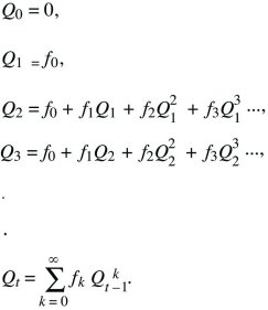
It is simplest to assume that individuals reproduce only once, and in synchrony, so that time can be counted in discrete generations. Each individual leaves 0, 1, 2, ... offspring with probability f0, f1, f2, ... . Clearly, f0 + f1 + f2 + ... = 1, and the mean offspring number (i.e., the mean fitness) is

On average, the population is expected to grow by a factor  every generation, and by t over t generations. Indeed, the size of a very large population would follow the smooth and deterministic pattern of geometric increase as modeled above. However, this average behavior is highly misleading when numbers are small. The number of offspring of any one individual has a very wide distribution, with a high chance of complete extinction (Fig. 28.20). every generation, and by t over t generations. Indeed, the size of a very large population would follow the smooth and deterministic pattern of geometric increase as modeled above. However, this average behavior is highly misleading when numbers are small. The number of offspring of any one individual has a very wide distribution, with a high chance of complete extinction (Fig. 28.20).
What is the probability that after t generations, one individual will leave no descendants (Qt) or some descendants (Pt; necessarily Qt + Pt = 1)? Initially, this is Q0 = 0, because one individual must be present at the start (t = 0). The chance of loss after one generation is the chance that there are no offspring in the first generation, that is, Q1 = f0. To find the solution for later times, sum over all possibilities in the first generation. There is a chance f0 of no offspring, in which case loss by time t is certain. There is also a chance f1 of one offspring, in which case loss by time t is the same as the chance that this one offspring leaves no offspring after t – 1 generations. More generally, if there are k offspring, the chance that all k will leave no offspring after the remaining t – 1 generations is just  . Thus, a recursion allows us to calculate the chance of loss after any number of generations: . Thus, a recursion allows us to calculate the chance of loss after any number of generations:
This solution is shown in Figure 28.21, assuming a Poisson distribution of offspring number. If the mean fitness is less than or equal to 1 ( ≤ 1), extinction is certain. However, if the mean fitness is greater than 1, there is some chance that the lineage will establish itself, to survive and grow indefinitely. To find the chance of ultimate survival, find when Qt converges to a constant value, so that Qt = Qt – 1 = Q. This gives an equation for Q that can be solved either using a computer or graphically (Fig. 28.22). With binary fission, for example, an individual either dies or leaves two offspring (i.e., f0 + f2 = 1). Thus,
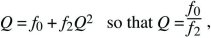
where the solution is only valid (Q < 1) if f0 < f2, which must be true if the population is to grow at all. If the distribution of offspring number is Poisson, with mean λ > 1, then
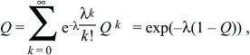
where the fact that
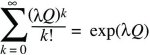
is used. The solution to this equation is shown graphically in Figure 28.22. For a growth rate of λ = 1.2, the probability of ultimate loss is Q ~ 0.686.
Usually, our concern is with the fate of alleles that have a slight selective advantage ( = 1 + s, where s << 1). There is a simple approximation that does not depend on the (usually unknown) shape of the distribution of offspring number, fk:

This remarkably simple result shows that when an allele has a small selective advantage s, its chance of surviving is twice that advantage divided by the variance in numbers of offspring, var(k). (With a Poisson number of offspring, var(k), the variance of offspring number is equal to its mean, which is = 1 for a stable population; thus, P = 2s.) The consequences of this relation are considered on pages 489–490.
The Sum of Many Independent Events Follows a Normal Distribution
The phenotype of an organism is the result of contributions from many genes and many environmental influences; the location of an animal is the consequence of the many separate movements that it makes through its life; and the frequency of an allele in a population is the result of many generations of evolution, each contributing a more or less random change. To understand each of these examples quantitatively, the combined effects of many separate contributions must be considered. Often, the overall value can be treated as the sum of many independent effects. If no effect is too broadly distributed, then the sum follows an approximately Gaussian distribution. This is known as the Central Limit Theorem and is illustrated in Figure 28.23 by an ingenious device designed by Galton.
Figure 28.24 illustrates this convergence to a Gaussian distribution and shows the distribution of each individual random effect. Although the distributions are initially quite different, and far from Gaussian, the distribution of their sum becomes smoother and converges rapidly to a Gaussian distribution. Necessarily, the distribution of the sum of two or more Gaussians is itself a Gaussian.
The mean of the overall distribution is the sum of the separate means, and the variance of the overall distribution is the sum of the separate variances. Because the shape of a Gaussian distribution is determined solely by its mean and variance, all other features of the component distributions are irrelevant. This is an important simplification, because it means that the process can be described in terms of just two variables—namely, the mean and variance of the component distributions. This is used elsewhere in the book to simplify our description of quantitative variation (p. 385) and that of the flow of genes through populations (Fig. 16.3).
Random Walks Can Be Approximated by Diffusion
The sum of a large number of independent random variables tends to a Gaussian distribution. We can think of this convergence as occurring over time. For example, consider an individual moving in a random walk so that its position changes by a random amount every generation. At any time, it will be at a random position drawn from a distribution that converges to a Gaussian. (To be more concrete, think instead of a population of randomly moving individuals and follow the distribution of all of them.) In this section, we show how the probability distribution changes approximately continuously in time, and can be described by a diffusion equation. This parallels our discussion of deterministic models, where it was shown that a variety of different models of evolution can be approximated by a differential equation in continuous time. Similarly, a range of random models can all be approximated by a diffusion of the probability distribution. This gives a powerful method for understanding the interaction between different evolutionary processes.
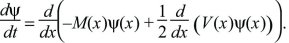
Consider a variable x, which has distribution ψ(x, t) at time t. If the changes in each time step are small and have constant mean M and variance V, then the distribution spreads out according to a differential equation that gives the rate of change of the distribution, dψ/dt (Box 28.6). If the population starts out concentrated at a single point (or the position of a single individual that starts at that point is considered) then the solution is a Gaussian distribution with mean Mt and variance Vt (Fig. 28.25, left column). Other initial distributions lead to different solutions. A sharp step decays in a sigmoidal curve (Fig. 28.25, middle column), whereas sinusoidal oscillations decay at a steady rate, proportional to the square of their spatial frequency (Fig. 28.25, right column). The effect of diffusion is to smooth out distributions over time.
Box 28.6 The Diffusion Approximation
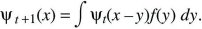
Suppose that at time t, a variable x has distribution ψt(x); x might represent the position of a randomly moving individual or the allele frequency in a randomly evolving population. In the next generation, a small random quantity y is added, giving a new and broader distribution, ψt + 1(x). The probability of finding x at time t + 1 is the chance that the value was x – y at time t, and that the additional perturbation was y. Averaging over the distribution of perturbations, f(y):
Now, assume that the distribution ψt is smooth, and much broader than the distribution of perturbations, f(y). Then, ψt(x – y) can be approximated as
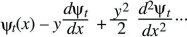
(This is known as a Taylor’s series approximation [Fig. 28.26].) It can be shown that as long as f(y) is not too broad, only the terms shown here are needed, involving the gradient (dψt/dx) and curvature (d2ψt/dx2), just as, when the Central Limit Theorem holds, only the mean and variance are needed to describe the distribution. Substituting into the integral above,
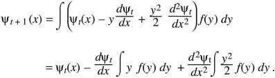
Finally assume that changes from one generation to the next are small, so that ψt + 1 – ψ t can be approximated by the continuous rate of change dψ/dt. If the mean perturbation is written as
∫ y f(y) dy = M,
and the mean square perturbation (which is approximately equal to the variance for small M) as
∫ y2 f(y) dy = V,
then
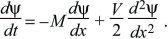
If the distribution is initially concentrated as a sharp spike at x = 0, then the solution to this diffusion equation is a Gaussian with mean Mt and variance Vt (Fig. 28.25, left column).
In this derivation, it is assumed that the distribution f(y) and hence M and V are constant. In general, they will depend on x and can be written as M(x), V(x). Then, the formula given in the main text applies.
When the mean and variance (M, V) of each small fluctuation are fixed, the distribution follows a Gaussian (Box 28.6). Thus, the simple case is really a different way of presenting the Central Limit in terms of differential equations. In general, however, the mean and variance of changes in each generation will depend on the state of the system, in which case the distribution will almost always not be Gaussian. For example, changes in allele frequency must decline to 0 as allele frequencies tend to 0 or 1, because they must remain within these bounds. The successive changes are then no longer independent of each other, and the Central Limit Theorem no longer applies. However, the change in the distribution can still be described by a diffusion equation, which is a straightforward extension of that derived in Box 28.6:
This differential equation is extremely important in population genetics, because it gives a simple way to analyze the effects of different evolutionary processes on the distribution of allele frequencies (e.g., see Box 28.7) The neutral theory of molecular evolution (p. 59) was largely based on this method for analyzing the effects of random fluctuations; additional examples are on pages 495–496 and 641.
Box 28.7 Selection and Migration in a Small Population
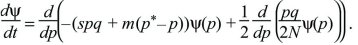
The diffusion equation is a powerful tool for finding how different evolutionary processes combine. For example, imagine that an allele P is favored by selection s in a small population of N diploid individuals. However, polymorphism is maintained by immigration at rate m from a larger population with allele frequencies q* and p*. In this model, the mean change of allele frequency per generation is M(p) = spq + m(p*– p) and the variance of fluctuations in allele frequency caused by random drift is V(p) = pq/2N (Box 15.1). Substituting these into the diffusion equation in the main text, the rate of change of the distribution of allele frequency is
The probability distribution will reach an equilibrium where dψ/dt = 0. (If there are many subpopulations, then this will be the distribution of allele frequency across the entire set.) This equilibrium can be found by setting
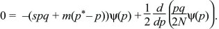
This can be rearranged to give a formula in terms of pqψ:
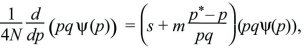
which can be integrated to give a solution
ψ = C p4Nmp*–1q4Nmq*–1 exp(4Nsp),
where the constant C is chosen so that the probability sums to 1. (This solution can be verified by substituting it back into the diffusion equation.)
The most important feature of this distribution is that it depends only on the scaled parameters Nm and Ns, which give the strength of migration and selection relative to drift. When Ns is large, selection can maintain the favored allele P at high frequency, so that the distribution is peaked at the right. When Nm is small, the population tends to be fixed for one or the other allele (Fig. 28.27A), whereas when it is large, the distribution is pulled toward the frequency in the migrant pool (p ~ p*) (Fig. 28.27B).
Summary
Mathematical theory is widely used in evolutionary biology, both to understand how populations evolve forward in time and to make inferences from samples of genes traced back through time. Models of deterministic processes, such as selection, mutation, recombination, and migration, follow the proportions of different genotypes through time. In sexually reproducing populations, this is difficult with more than a few genes, because of the huge number of possible gene combinations. Reproducing populations tend to grow exponentially; a variety of models, evolving either in discrete generations or continuously, can be approximated by a simple differential equation. Differential equations involving a single allele frequency can be solved, but scaling arguments can be used in more complex cases to show that the outcome depends only on parameter combinations such as the ratio of migration to selection, m/s. Models can be understood by identifying their equilibria and by finding whether these equilibria are stable. Near to equilibria, the model can be approximated by simple linear equations, and its behavior depends on the magnitude of the leading eigenvalue. The concept of probability is crucial both for following the proportions of different genotypes in deterministic models and for understanding the random evolutionary process of genetic drift. The probability distribution describes the chance of any possible outcome and may be defined for discrete possibilities (e.g., the numbers of individuals) or for continuous variables (spatial location or allele frequency in a large population, say). We describe two important models for how probability distributions change through time: branching processes, which apply to populations of genes or individuals that reproduce independently of each other, and the diffusion approximation, which applies when random fluctuations are small.
Further Reading
Hacking I. 1975. The emergence of probability. Cambridge University Press, Cambridge.
A nice history of ideas in probability and statistics; useful to thoroughly understand the basic concepts of probability.
Haldane J.B.S. 1932. The causes of evolution. Longmans, New York.
This classic account includes an appendix that gives a concise summary of the basic models of population genetics.
Otto S.P. and Day T. 2007. A biologist’s guide to mathematical modeling in ecology and evolution. Princeton University Press, Princeton, New Jersey.
An excellent introduction to both deterministic and stochastic models in ecology and evolution.
|